Sensitivity and reliability analysis of tower cranes
As part of CIVL 492: Directed Studies (under the supervision of Dr. Terje Haukaas), this project focuses on the sensitivity and reliability analysis of tower cranes. The research examines how variations in loads, material properties, and structural configurations influence performance and safety. Probabilistic methods and computational modeling are applied to identify critical parameters and provide insights for reliability-based design.
Sensitivity Analysis
For the scope of this study, Sensitivity Analysis is defined as the derivative of a structural response quantity with respect to an input parameter. If the structural response is denoted by (e.g., displacement), and the input parameter is , then the first-order sensitivity is expressed as

where “x” may represent any model parameter, including yield strength, elastic modulus, cross-sectional area, geometric dimensions, or applied loads.
First-order sensitivity represents the change in the structural response for a unit change in the input parameter of interest. It quantifies how strongly the model output reacts to small perturbations in that parameter while all others are held constant.
Second-order sensitivity is defined as the second derivative of the response with respect to one or more input parameters. For example,

represents the interaction effect between parameters “Xi” and “Xj”. It measures how the first-order sensitivity with respect to one parameter changes when another parameter is varied. In other words, second-order sensitivity captures the combined effects between model inputs.
A sensitivity study can be used to identify which input parameters exert the greatest influence on the structural response of the tower crane model. However, first-order sensitivities alone cannot be used to rank parameters directly in terms of importance because they retain the physical units of the derivative. For example, the modulus of elasticity “E” is measured in Pascals, whereas an applied force is measured in Newtons. Since the derivatives carry different units, a direct numerical comparison does not provide a meaningful measure of relative importance.
To enable comparison across parameters, the sensitivities may be scaled by the standard deviation of the corresponding random variable. This produces a normalized measure of influence:

Multiplying by the standard deviation effectively normalizes the units and reflects the contribution of each parameter’s uncertainty to the overall variability in the structural response. These normalized sensitivities provide a consistent basis for comparing the relative influence of different input parameters within the model.
For a linear elastic structural system, the governing equilibrium equation may be written as

Where K is the global stiffness matrix, U is the displacement vector, F is the external load vector, and x represents a model parameter
The stiffness matrix, displacement vector, and load vector all depend on the parameter x in the governing equation, differentiation with respect to x gives:

Rearranging, the below expression provides the first-order sensitivity of the displacement vector with respect to the parameter x

Reliability Analysis
Definition of Reliability
In structural reliability analysis, the reliability of a system is defined as:

The probability of failure is expressed as:

where g(x) is the limit state function, and x is the vector of random variables describing the system (e.g., modulus of elasticity, cross-sectional area, yield strength, applied load, etc.).
Failure occurs when the limit state function becomes less than or equal to zero. Therefore, the probability of failure represents the probability that the system response exceeds the prescribed failure threshold.
Limit State Function Formulation
The limit state function g(x) defines the boundary between safe and failed states. It must be formulated such that:

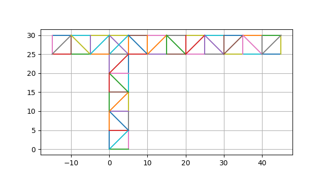
Application to the Tower Crane Model
For the tower crane structural model, the response quantity of interest is the vertical displacement at a selected node under a point load .
In the analysis program, downward displacement is considered negative. If the limit state function were defined directly as:

where u is the vertical displacement, then any downward displacement would immediately produce a negative value of g(x). This would result in failure at the mean realization of the random variables.
To establish a meaningful failure threshold, the limit state function is instead defined as:

In this formulation, failure is defined as occurring when the vertical displacement exceeds -1.7m at the node of interest.
For displacements more negative than -1.7m, the limit state function becomes negative, indicating failure. The value of 1.7 m was selected based on observed nodal displacement magnitudes from the structural model. It serves as a prescribed displacement limit to evaluate the reliability of the system and provides a defined performance boundary that allows computation of the probability of failure.
SAMPLE PARAMETRIC CODE
from G2AnalysisNonlinearStatic import *
from G2Model import *
import matplotlib.pyplot as plt

from G2Model import *
from G2Example17_b_parameters import *

def structuralModel(names, x):

    # Pick up values for the random variables
    for i in range(len(x)):
        exec("global %s; %s = %.22e" % (names[i], names[i], x[i]))
    # -----------------------------------------
    # Global parameters
    # -----------------------------------------
    elementType   = 2
    materialType  = 'Bilinear'  # 'Bilinear'/'Plasticity'/'BoucWen'

    P             = 30000
    #A             = 1.4192e-03
    E             = 200e9
    fy            = 350e16
    alpha         = 0.05

    #I = (A**2)/12 # Square Sections
    # Circular Sections
    #d = np.sqrt(4.0 * A / np.pi)
    #I = np.pi * d**4 / 64.0

    #Hollow Circle
    Do = 0.0552
    Di = 0.0352
    A = (np.pi/4.0) * (Do**2 - Di**2)
    I = (np.pi/64.0) * (Do**4 - Di**4)

    nsteps        = 3
    dt = 1/nsteps
    KcalcFrequency= 1
    maxIter       = 100
    tol           = 1e-5


    def build_crane(Hm=50.0, Lj=75.0, Lc=25.0, panelWidth=5.0, panelHeight=5.0):
        """
        Panel Based Tower Crane Breakdown:
        - Mast: n_mast vertical panels
        - Main jib: n_jib panels to +x
        - Counter-jib: n_cj panels to -x

        NODES: [[x coordinate,y coodinate], ...]
        ELEMENTS: [elementType, preAxialForce, nodeI_ID, nodeJ_ID]

        """

        # Number of panels
        n_mast = int(round(Hm / panelHeight))
        n_jib  = int(round(Lj / panelWidth))
        n_cj   = int(round(Lc / panelWidth))

        NODES    = []  # 0-based
        ELEMENTS = []  # 1-based node IDs

        def add_node(x, y):
            """Append node"""
            NODES.append([float(x), float(y)])
            return len(NODES)-1

        def add_el(i_idx, j_idx):
            """Append element"""
            if i_idx != j_idx:
                ELEMENTS.append([elementType, 0.0, i_idx + 1, j_idx + 1])

        # -------------------------------------
        # 1) MAST
        # Node pattern (0-based):
        #   level k (0..n_mast) → left = 2*k, right = 2*k+1
        # -------------------------------------

        # Base level k = 0
        NODES.append([0.0,        0.0])        # node index 0 (left)
        NODES.append([panelWidth, 0.0])        # node index 1 (right)

        # Base Level Horizontal Chord?
        #add_el(0,1)

        # Levels k = 1..n_mast
        for k in range(1, n_mast + 1):
            yk = k * panelHeight

            # New nodes at this level
            NODES.append([0.0,        yk])    # index 2*k
            NODES.append([panelWidth, yk])    # index 2*k+1

            topL = 2*k
            topR = 2*k + 1
            botL = 2*(k-1)
            botR = 2*(k-1) + 1

            # vertical chords
            add_el(botL, topL)
            add_el(botR, topR)

            # top horizontal
            add_el(topL, topR)

            # diagonals (X-shaped)
            add_el(botL, topR)
            add_el(botR, topL)

        # Mast indices (0-based)
        mast_top_left_idx        = 2 * n_mast
        mast_top_right_idx       = 2 * n_mast + 1
        mast_left_below_top_idx  = 2 * (n_mast - 1)
        mast_right_below_top_idx = 2 * (n_mast - 1) + 1

        # -------------------------------------
        # 2) MAIN JIB (to the right, +x)
        # -------------------------------------
        jib_top_indices = [mast_top_right_idx]
        jib_bot_indices = [mast_right_below_top_idx]

        for j in range(1, n_jib + 1):
            xj    = panelWidth + j*panelWidth
            y_top = n_mast * panelHeight
            y_bot = (n_mast - 1) * panelHeight

            nb_idx = add_node(xj, y_bot)  # new bottom
            nt_idx = add_node(xj, y_top)  # new top

            jib_bot_indices.append(nb_idx)
            jib_top_indices.append(nt_idx)

            botL = jib_bot_indices[-2]
            topL = jib_top_indices[-2]
            botR = jib_bot_indices[-1]
            topR = jib_top_indices[-1]

            # chords
            add_el(topL, topR)
            add_el(botL, botR)

            # vertical
            add_el(botR, topR)

            # alternating diagonals
            if j % 2 == 1:
                add_el(botL, topR)   # odd: bottom-left → top-right
            else:
                add_el(topL, botR)   # even: top-left → bottom-right

        tip_top_idx = jib_top_indices[-1]   # 0-based

        # -------------------------------------
        # 3) COUNTER-JIB (to the left, -x)
        # -------------------------------------
        cj_top_indices = [mast_top_left_idx]
        cj_bot_indices = [mast_left_below_top_idx]

        for j in range(1, n_cj + 1):
            xj    = -j * panelWidth
            y_top = n_mast * panelHeight
            y_bot = (n_mast - 1) * panelHeight

            nb_idx = add_node(xj, y_bot)
            nt_idx = add_node(xj, y_top)

            cj_bot_indices.append(nb_idx)
            cj_top_indices.append(nt_idx)

            botR = cj_bot_indices[-2]   # toward mast
            topR = cj_top_indices[-2]
            botL = cj_bot_indices[-1]   # farther left
            topL = cj_top_indices[-1]

            # chords
            add_el(topR, topL)
            add_el(botR, botL)

            # vertical
            add_el(botL, topL)

            # mirrored alternating diagonals
            if j % 2 == 1:
                add_el(botR, topL)   # odd: bottom-right → top-left
            else:
                add_el(topR, botL)   # even: top-right → bottom-left

        # -------------------------------------
        # 4) CONSTRAINTS
        # -------------------------------------
        CONSTRAINTS = [[0, 0] for _ in NODES]
        CONSTRAINTS[0] = [1, 1]   # base left
        CONSTRAINTS[1] = [1, 1]   # base right

        # -------------------------------------
        # 5) LOADS (0-based like NODES)
        # -------------------------------------
        LOADS = [[0.0, 0.0] for _ in NODES]
        LOADS[tip_top_idx][1] -= P   # downward load at jib tip (top chord)

        # -------------------------------------
        # 6) SECTIONS & MATERIALS
        # -------------------------------------
        nel = len(ELEMENTS)
        SECTIONS  = [['Truss', A] for _ in range(nel)]

        MATERIALS = []
        for _ in range(nel):

            MATERIALS.append(['Bilinear', E, fy, alpha])


        return NODES, CONSTRAINTS, ELEMENTS, SECTIONS, MATERIALS, LOADS, tip_top_idx


    # -------------------------------------------------
    # Build model and run analysis
    # -------------------------------------------------
    Hm, Lj, Lc      = 10.0, 25.0, 5.0
    panelWidth      = 1.2
    panelHeight     = 1.2

    NODES, CONSTRAINTS, ELEMENTS, SECTIONS, MATERIALS, LOADS, tip_idx = build_crane(
        Hm=Hm, Lj=Lj, Lc=Lc, panelWidth=panelWidth, panelHeight=panelHeight
    )

    trackNode = tip_idx   # 0-based index in NODES
    trackDOF  = 2         # vertical DOF

    MASS = [[0.0, 0.0] for _ in NODES]
    input_data = [NODES, CONSTRAINTS, ELEMENTS, SECTIONS, MATERIALS, LOADS, MASS]
    m = model(input_data)

    DDMparameters = [
        ['Element', 'A',     [52]],
        ['Element', 'A',     [108]],
        ['Element', 'A',     [2]],
        ['Element', 'A',     [1]]
    ]
    plotFlag = False
    t, loadFactor, u, dudx, ddm2 = nonlinearStaticAnalysis(m, nsteps, dt, maxIter, KcalcFrequency,tol, trackNode, trackDOF, DDMparameters, plotFlag)
    if plotFlag:
        plt.ion()
        plt.figure()
        plt.autoscale(True)
        plt.plot(t, dudx[0, :], 'k-')
        plt.plot(t, dudx[1, :], 'r-')
        plt.plot(t, dudx[2, :], 'g-')
        plt.plot(t, dudx[3, :], 'b-')
        #plt.ylabel('Sensitivity at jib tip (DOF 2)')
        plt.grid(True)

        print("\nClick somewhere in the plot to continue...")
        print("Buckling Load: ", ((np.pi**2) * E * I)/(panelWidth**2))
        print("Axial Load: ", (A*fy))
        plt.waitforbuttonpress()